Custom error bars can be applied either in Fully Automatic Mode or in Interactive Mode. The latter, described below, allows you to indicate a range of cells where the error data is located.
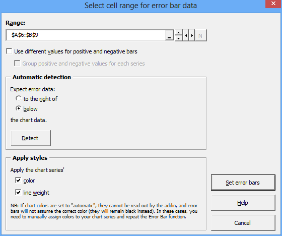
In the Interactive Mode dialog, select the range of cells that contain your error values. You can use the arrow buttons to move the selected range over the spreadsheet, or click “Auto” to reset the range to the automatically determined range either to the right of or below the chart data, depending on your settings.
You can also indicate whether you want the chart series color and line formatting to be applied to the error bars. Note however that ‘automatic’ colors and lines, which Excel applies by default to new charts, cannot always be read by the XL Toolbox (read more).
Independent values for ‘plus’ and ‘minus’ bars
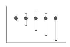
Starting with Toolbox version 2.72, error bars can be set to independent positive and negative values. You need to use the “Interactive error bars” function to accomplish this.
To make the Toolbox apply independent positive and negative error bars, tick the “Use different values…” checkbox:
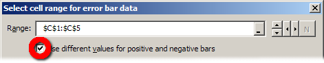
The Toolbox will then expect the ‘positive’ values in the first row or column of the selected cell range, and the ‘negative’ values in the column to the right or the row below, depending on the orientation of your data.
Note: For the sake of ease of use, it is not necessary to define a range of two rows or columns. Simply select the cells that contain the positive values, the negative values will automatically be taken from the column to the right or the row below.