The Group Allocation function serves to assign study subjects to treatment groups, minimizing differences between the treatment groups. This is also called stratification. The study subjects can have as many properties/characteristics (e.g. body weight, age, etc.) as you like or as is reasonable.
How to use the Group Allocator
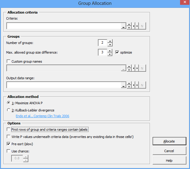
When you use the Group Allocator, you have to enter a number of parameters:
-
Allocation criteria: This is a range of cells in your spreadsheet that contains the criteria that you want to base the allocation on. In the simplest case, this would be a vertical range of cells containing e.g. body weights or age. If you want to have several criteria, e.g. body weight, age, and blood pressure, you need to have those values in several columns.
-
Number of groups: Indicate how many treatment groups you want to have.
-
Max. allowed group size difference: The allocation algorithm will primarily assign subjects based on their characteristics, which may result in treatment groups that are very similar, but contain different numbers of subjects. You can indicate here what size difference you want to tolerate.
-
Optimize: When checked, the Allocation function will play with the Group size difference and find the best setting that still fulfills the limit you set. In most cases, you want to make use of this option. If it is unchecked, the algorithms will work strictly with the size difference limit that you set, which may lead to a less effective allocation.
Optimize is not compatible with the Use chance option.
-
Custom group names: If you want, you can use your own group names.
If checked, you need to indicate a range of cells that contains your own group names. If unchecked, standard group names will be used (“Group A”, “Group B”, etc.). -
Allocation method: You can select one of two algorithms: either “ANOVA P” method or “Kullback-Leibler divergence”. See below for an explanation.
-
Pre-sort: When checked, the study subjects will be sorted according to the allocation criteria before the group assignment starts. This improves the outcome, but is slower.
-
Use chance: If you want, you can introduce an element of chance into the allocation process. Enter a number between 0.01 and 0.99 in the box to the right. For example: If you enter 0.9 here, a subject will be assigned the computed treatment group only with a 90 % chance.
Use chance is not compatible with the Optimize option.
-
First row of group and critera ranges contain labels: Self-explanatory; has no consequence for your allocation. This options just serves to make range selection more convenient.
-
Write p values underneath criteria data: If checked, an analysis of
variance will be performed after the allocation process, and the resulting p values for each allocation criterion will be written underneath the corresponding cells. Note that any existing data in those cells will be overwritten without notice.
Overview of allocation methods
The Group Allocation function offers two different computation algorithms: The “Maximize ANOVA P” method and the “Kullback-Leibler divergence” method.
Both algorithms start by priming the treatment groups, i.e. they arbitrarily assign a certain number of subjects to the treatment groups. Then, they iterate through each of the remaining subjects and simulate assigning the subject to each of the treatment groups. From this simulation, the “best” treatment group for this subject is determined by computation, and subsequently the subject is assigned to that group.
Note: An important difference between the two algorithms is that the “ANOVA P” method can allocate any reasonable number of study groups. The “KLD” method on the other hand always allocates to two groups and allocation to a higher number of groups is achieved by recursing through previously allocated groups. Therefore, the “KLD” method can only allocate to 2, 4, 8, 16, … groups (power of 2).
Algorithm 1: Maximize ANOVA P
The “ANOVA P” algorithm work as follows: First, it arbitrarily assigns one subject to each group. Then, it iterates through the remaining subjects. Each subject is temporarily assigned to each study group, and the resulting p values of an analysis of variance for all allocation criteria are calculated. The p values are summarized for all criteria, and the subject is finally assigned to the treatment group that will result in the highest sum of P, but only if by assigning the subject to that group, the difference in group sizes does not exceed the user-defined limit (see above). If it does exceed the allowable size difference, the subject is assigned to the smallest group.
Algorithm 2: Kullback-Leibler divergence (KLD)
The Kullback-Leibler divergence (KLD) algorithm is based on a publication by Endo et al. (Contemp Clin Trials 2006;27:420, doi:10.1016/j.cct.2006.05.002).
It works as follows: First, it arbitrarily assigns two subjects to each group. Then, it iterates through the remaining subjects. Each subject is temporarily assigned to each study group, and the resulting KLD for the groups is computed. (A KLD is basically a measure for the difference between two distributions; read more in Wikipedia).
The subject is assigned the treatment group that will result in the smallest KLD, hence the smallest difference between the distributions.
This works only for two groups. If a higher number of treatment groups is needed, the function has to recurse through the previously allocated groups and split them in two. Therefore, the user-entered number of groups, when using the KLD algorithm, must be a power of two (2, 4, 8, 16, and so on).
Comparison of the two algorithms
It is up to the user to determine which algorithm works best for the task at hand.
To get an idea how the algorithms compare, allocations with real subjects were performed. Data of 40 mice were entered into a spreadsheet, and the Group Allocation was performed six times with the two algorithms, using one criterion each time. The criteria were: Body weight, area under the curve for an insulin tolerance test, and relative fat mass. The number of treatment groups was “2” or “4”. The maximum allowed group size difference was always “2”.
The following figure shows the resulting six p values of an analysis of variance as a correlation of both algorithms.
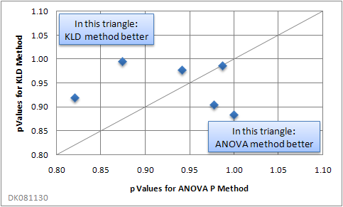
When using two or more allocation criteria, there was a tendency for the “ANOVA P” method to yield better results:
| Algorithm that resulted in higher p values | |||
|---|---|---|---|
| No. of criteria | |||
| No. of groups | 1 | 2 | 3 |
| 2 | (None) | KLD | ANOVA P |
| 4 | ANOVA P | ANOVA P | ANOVA P |
Your results will of course vary, depending on your actual data.
Note that a high P value does not necessarily imply perfect distribution. P values derived from an ANOVA are the higher, the greater the variability within the groups compared with the variability of the group means is. Thus, an “ugly” distribution of data points within groups may result in a high P value, even though the allocation result is far from perfect. If perfect allocation, e.g. utmost equality of distributions in the groups, is important, it is recommended to compare both allocation methods with and without pre-sorting.
Limitations
There are a few limitations to both algorithms:
- Subjects are not permutated, i.e. the order of the study subjects matters. It is possible that group allocations is different if you change the order of your study subjects. (Version 2.10 of the XL Toolbox introduces the “Pre-sort” option that improves the allocation outcome.)
- You cannot use criteria with nominal data, e.g. gender or color names.
- The KLD algorithm only works with group numbers that are powers of 2 (for an explanation see above).
Group Allocation: A pracical example
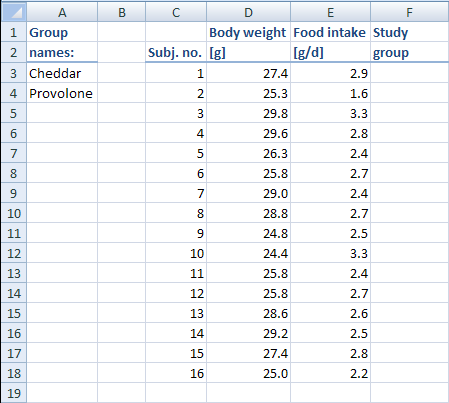
Here is an example to illustrate the Group Allocation function with a practical example. Let’s suppose you have a large family of mice in your kitchen that you are friendly with and that agree to participate in a study. The study will involve dividing them in several groups that get fed one type of cheese; you measure their body weight, and at the end of the study you want to know which cheese makes the mice the fattest.
When assigning your friends to the “treatment” groups, you want to make sure that there are no differences in body weight at the outset. Also, because you know that some individuals generally eat more than others, you want your treatment groups to be similar with respect to the daily food intake.
First, arrange the data so that the body weights and the food intake are each in their own column:
Then, start the Group Allocator from the menu (Excel® 2003) or from the Ribbon (Excel® 2007) and enter the following parameters:
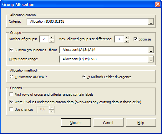
As you can see in the screenshot above, we have chosen in this particular example to make use of our own group names.
When you click on “Allocate”, the subjects will be assigned a “treatment”, in this example a type of cheese that they are going to eat in the study. The result looks as follows:
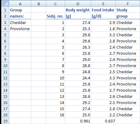
Since we chose to have the P values written underneath the columns that contain the allocation criteria, we can easily see how well the allocation worked. If there were absolutely no differences between the two groups, the P values would be 1. The body weights come quite close (p = 0.961), but the food intake data is not as well distributed.
Allocation/randomization
Citations
Kranz, L. M. (2016) Systemic RNA delivery to dendritic cells exploits antiviral defence for cancer immunotherapy. Nature.
Kreiter, S. et al. (2015) Mutant MHC class II epitopes drive therapeutic immune responses to cancer. Nature.
Framroze, B. et al. (2015) A Comparative Study of the Impact of Dietary Calcium Sources on Serum Calcium and Bone Reformation Using an Ovariectomized Sprague-Dawley Rat Model. Journal of Nutrition & Food Sciences, 5, 348.